Analysis
Selection and queries
Map › Select picks features by clicking or dragging a box (Shift adds, Ctrl removes). Select By Attributes takes a SQL clause and checks it as you type; Select By Location picks features that touch another layer's features or lie within a search distance of them (or, inverted, those that don't). Selected features draw in cyan and are highlighted in the attribute table, and the selection is synced both ways. Switch, clear or zoom to the selection, or make a new layer from it.
Select By Attributes and definition queries use SQL WHERE clauses:
pop_est > 100000000 AND continent = 'Asia'
name LIKE 'S%'
iso_a3 IN ('FRA', 'DEU', 'ITA')
gdp_md IS NULL
"OR" = 1          -- double quotes name a field, even a keyword
Geoprocessing tools
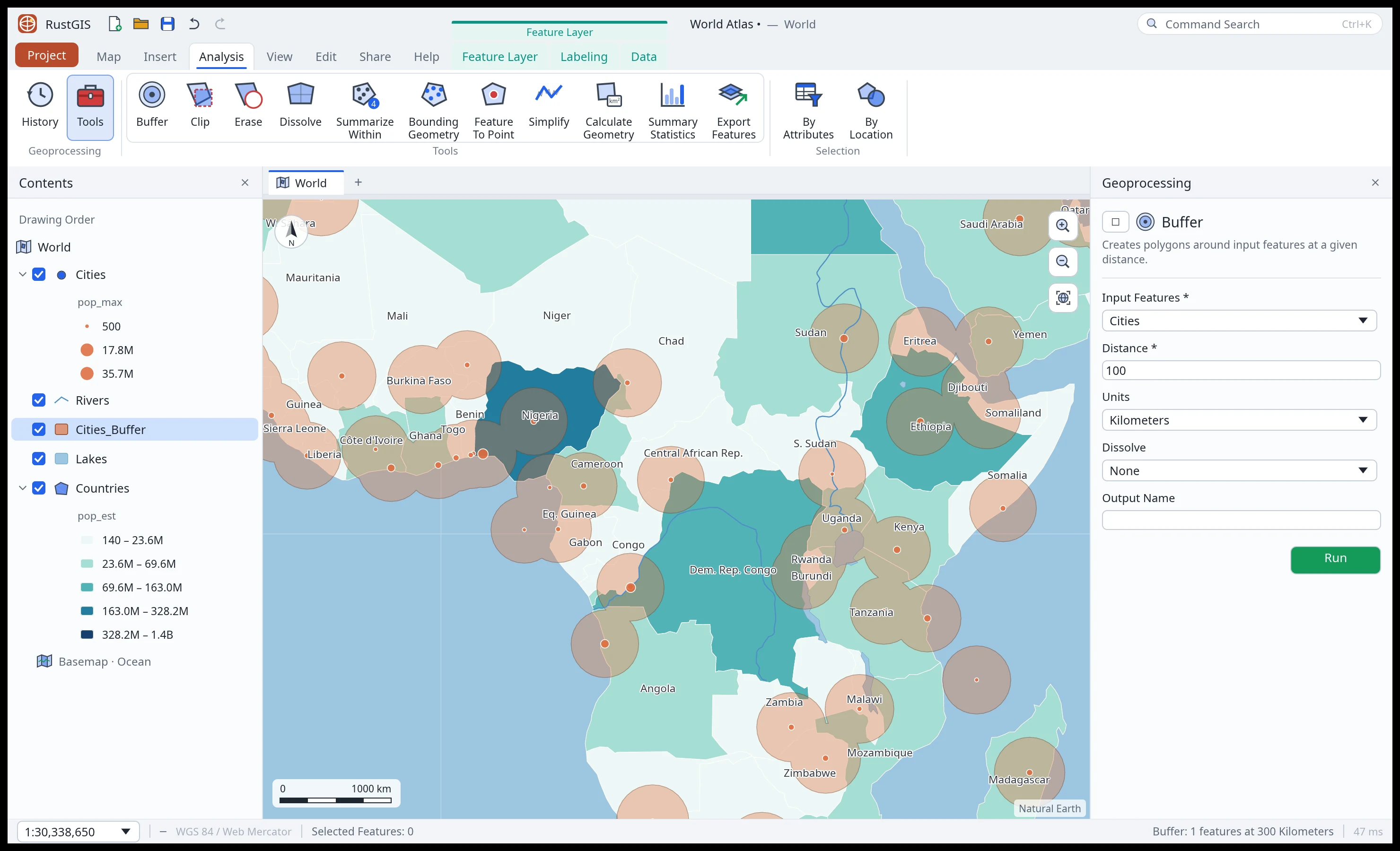
Open a tool from the Analysis tab's gallery, Analysis › Tools (the Geoprocessing pane, which searches every tool) or Command Search. Fill in its parameters and click Run: the result is added to the map, and the run is listed under Analysis › History. The built-in tools:
| Tool | Toolbox |
|---|---|
| Buffer | Analysis › Proximity |
| Clip, Erase | Analysis › Extract / Overlay |
| Dissolve | Data Management › Generalization |
| Minimum Bounding Geometry, Feature To Point, Calculate Geometry Attributes | Data Management › Features |
| Simplify | Cartography › Generalization |
| Select Layer By Location / Attribute | Data Management › Layers and Table Views |
| Summarize Within, Summary Statistics | Analysis › Summarize / Statistics |
| Export Features | Conversion |
Tools honour the current selection: with features selected, only those are processed.
GeoLibre tools
The desktop app and the command line can also run the GeoLibre tool suite: over 1,000 tools from Whitebox and GeoLibre for terrain analysis (slope, aspect, hillshade, curvature), hydrology (fill depressions, flow direction and accumulation, watersheds), image processing, interpolation and vector work. They run on the map's layers and add their outputs as new layers.
The suite is an optional download, so RustGIS itself stays small: the GeoLibre runner, a
single geolibre program (about 20 MB to download). In the Geoprocessing pane, click
Install GeoLibre tools under GeoLibre tools: RustGIS downloads the latest runner for your
platform from the geolibre-rust releases,
checks it against its published SHA-256 checksum (which catches a corrupted download; the
release itself is trusted as when you download it by hand) and installs it in its data folder
(~/.local/share/rustgis/geolibre on Linux, ~/Library/Application Support/RustGIS/geolibre
on macOS, %LOCALAPPDATA%\RustGIS\geolibre on Windows). From the command line,
gp.installGeolibre does the same.
To install it yourself instead, download the archive for your platform
(geolibre-<version>-<platform>.tar.gz, or .zip on Windows), unpack it anywhere, and click
Locate… to pick the geolibre program; RustGIS remembers it.
RustGIS also finds the runner without asking when it is next to the RustGIS program (or in a
geolibre folder beside it), on your PATH, or named by the RUSTGIS_GEOLIBRE environment
variable (the command line uses these). The tools then appear under GeoLibre › Raster,
Vector, Lidar, Hydrology, Terrain, Conversion in the Geoprocessing pane and the Catalog's
toolboxes, and Find Tools searches them.
- Raster inputs are passed as their own files; vector layers (or their selection) are written in the first raster input's coordinate system, or the UTM zone around the data, so distances and areas are in metres. Data spanning more than 40° of longitude stays in degrees.
- Raster outputs are kept inside the project, so they save and reopen with it. Text and table reports appear in the tool's messages.
- LiDAR and other inputs RustGIS doesn't open as layers take a file path, read like Add Data reads one. Outputs are written to a fresh scratch folder and loaded from there.
- Each run is a separate
geolibreprocess, so a tool that fails can't take RustGIS down. - From the command line:
gp.run={"tool":"geolibre:slope","params":{"input":"dem"}};gp.toolslists every tool's parameters,gp.geolibreshows the runner in use andgp.setGeolibre={"path":"…"}picks one.
In the web app, click Load GeoLibre tools in the Geoprocessing pane instead. RustGIS
loads geolibre-rust's WebAssembly runner (the geolibre-wasm package, from jsDelivr, about
25 MB the first time, then from the browser's cache) and the tools run in the page, in an
in-memory folder: nothing is uploaded. The web app remembers this and loads them again on your
next visit. The runner's code comes from jsDelivr, pinned to one geolibre-wasm release, the
same trust as installing that package. Tools that read files by path (LiDAR files, for instance) need the desktop app,
since a web page has no file system.
In the desktop app and on the command line, RustGIS waits while a tool runs, so a long run on a large raster or point cloud keeps the window busy until it finishes. In the web app the run is started in the background and the result is added when it ends, but the tool itself runs in the page, so the page is busy while it computes.
Analysis workflows
The Analysis tab's Workflows pane holds guided analyses. Where one needs points, it asks you to click them on the map:
| Workflow | What it does |
|---|---|
| Raster Functions | Slope, aspect, hillshade, NDVI, band math ((b4-b3)/(b4+b3)), thresholds, resampling |
| Function Editor | Chains raster functions, each on the previous output |
| Suitability Modeler | Scores rasters 1–10 and adds them with weights |
| Visibility Analysis | A viewshed from a point on an elevation raster |
| Exploratory 3D Analysis | A line of sight between two points, split into seen and hidden parts |
| Geostatistical Wizard | An IDW surface from point values |
| Network Analysis | The shortest (or cheapest, by a cost field) route over a line layer |
| Neighborhood Explorer | What lies within a distance of a point, with sums of numeric fields |
| Simulation | Random points in polygons (a fixed number, or from a field × rate) |
| Data Engineering | Counts, nulls, distinct values, min, max and mean of every field |
| Exploratory Analysis | Histograms and correlations of numeric fields |
| Embeddings | The features most like the selected one, by their numeric attributes |
| Data Interop | KML, GPX, CSV with WKT, GeoJSON or CSV |
Rasters these make are kept in the project. Environments limit tools to the map view, the full
extent or everywhere, and set the cell size of new rasters. ModelBuilder chains tools into
models (a parameter %1 is step 1's output), and New Model From History turns the
geoprocessing you've run into a model. The Script pane runs commands from text, one per line
(id {json}).
Imagery
The Imagery tab opens its tools in the Workflows pane:
- Ortho Mapping and Reality Mapping workspaces mosaic georeferenced images into an orthomosaic, or elevation rasters into a surface model that exports as a 3D mesh (OBJ).
- Georeference places a raster from control points (column, row, longitude, latitude) or stretches it over the map view.
- Change Detection (difference, ratio, percent), Spectral Analysis (every band at a pixel), Indices (NDVI, NDWI, SAVI, NBR, NDBI, EVI), Process (clip to the view, resample) and the Pixel Editor (set the pixels inside a polygon).
- Classification Wizard (unsupervised k-means) and Classification Tools (minimum distance from training polygons).
- Mensuration: distances along the surface, heights between two points, areas, and volumes above or below a base height, with a list of results.
Deep learning and hosted imagery
Imagery › Deep Learning Tools trains a neural network (a multilayer perceptron) on the pixels under training polygons and classifies every pixel, adding a class raster with a confidence band and reporting the accuracy on held-back pixels. Trained models stay in the project; Share › Package › Deep Learning saves one as a package to apply in other projects. Imagery › Create Hosted Imagery cuts a raster into XYZ web map tiles (PNG, transparent outside the raster) with a TileJSON file and a viewer page.